Peanuts are a cash crop, particularly in China, India, Nigeria, the United States, and Sudan. The peanut crop is important due to its significant nutritional value, economic contribution to agriculture, and versatility in food products and industrial uses. For example, peanuts are used in the production of biodiesel, where peanut oil is converted into a renewable and eco-friendly fuel source. What could be more sustainable than driving a car fueled by biodiesel produced from peanuts?

To grow good yields of peanuts you must have good crop varieties and achieving this is one of the main tasks of peanut breeding. Current trends in peanut breeding focus on enhancing disease resistance, improving yield and quality traits, and incorporating advanced technologies like genomics and phenotyping for precise and efficient selection.

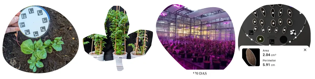
But, first, let’s start with peanut seed quality. To make proper data-driven decisions, you can use a free AI-powered mini-app Petiole Pro for quality assurance of peanut seeds. This app can provide information on the number of seeds, average seed area, diameter, and standard deviation. Additionally, there is an option for color assessment using different segmentation models.

Peanuts QA in Petiole Pro mobile platform helps with quality assurance of seeds, their count, size assessment and colour check

After considering the quality of your peanut seeds, it’s time to use breeding innovations, do proper monitoring of your crops, use drones for checking plant health and yield prediction and possess qualities from wild peanut relatives to improve disease resistance.

More details about peanut breeding and peanut farming are available in the research papers below and even better long-read is published here.

Optimizing Tropical Peanut Harvesting for Superior Seed Quality

Country: 🇧🇷 Brazil

Published: 08 May 2024

This study investigates the optimal harvest timing for tropical peanuts to achieve superior seed quality by examining the maturation stages and their impact on physiological and health parameters of the seeds.

The researchers utilized field-grown peanut plants (Arachis hypogaea L.) over two growing seasons (2021/2022 and 2022/2023) and monitored their development stages meticulously. They evaluated water content, dry weight, germination capacity, desiccation tolerance, vigor, longevity, and seed pathogens at various maturation stages (R5 to R9). Key techniques included oven drying for moisture analysis, germination tests under controlled conditions, accelerated aging tests, and principal components analysis (PCA) for data assessment. Statistical analysis was performed using ANOVA and Random Forest machine learning to identify significant variables impacting seed quality.

The study found that seeds harvested at late maturation stages (R7, R8, R9) exhibited higher vigour, longevity, and bioprotection against pathogens compared to those harvested earlier.

Notably, seeds at R7 had germination rates around 90%, while those at R9 achieved maximum performance with germination rates close to 100%. The Random Forest model highlighted normal seedlings, water content, and longevity as critical factors for assessing seed quality.

These findings are particularly useful for tropical peanut farmers and seed producers aiming to enhance seed quality and improve crop performance.

Main tools/technologies:

• High-throughput phenotyping
• Random Forest machine learning
• Controlled environment germination chambers
• Accelerated aging tests
• Principal components analysis (PCA)

For further details, refer to the research article by (Fonseca de Oliveira GR and Amaral da Silva EAA, 2024)[https://www.frontiersin.org/journals/plant-science/articles/10.3389/fpls.2024.1376370/full “Optimizing Tropical Peanut Harvesting for Superior Seed Quality in Brazil”].

Peanut seed production under field conditions. 1) Experimental area; 2) Opening of sowing furrows; 3) Open groove; 4) Sowing seeds; 5) Application of herbicide; 6) Seedling establishment at 10 days; 7) Fertilization at 30 days; 8) Peanut plants after 30 days; 9) Beginning of flowering; 10) Emission of the gynophores (pegs); 11) and 12) Application of fungicide and insecticide; 13) Weed management; 14) Plants at 100 days, when harvesting begins; 15) Harvesting carried out manually; 16) Washing fruits in pressurized water; 17) Classification of fruits; 18) Classification of seeds; 19 and 20) Drying the seeds; 21) Seed storage; 22) Seed analysis. Source: Fonseca de Oliveira GR & Amaral da Silva, 2024

Development and morphological changes of the fruit and seed of tropical peanut (Arachis hypogaea L., Virginia group, cultivar IAC 505) from flowering to full maturation (Crop season 2021/2022). Descriptions in chronological order for fruit/seed maturation: (A) one flower opened; (B) flower senescence after 24 h; (C) development of gynophore (peg) towards the soil; (D) peg penetrated the soil; (E) peg base begins its expansion; (F–K) fruit development in the soil; (L) Light Yellow fruit color/seeds in R5 stage; (M) Dark Yellow fruit color/seeds in R6 stage; (N) Yellow Brown fruit color/seeds in R7 stage; (O) Brown fruit color/seeds in R8 stage; (P) Black fruit color/seeds in R9 stage. Source: Fonseca de Oliveira GR & Amaral da Silva, 2024

Physiological quality of seeds. Crop season 2021/2022: (A) water content and dry weight; (B) germination capacity and desiccation tolerance; (C) radicle protrusion and time to 50% germination; (D) length of shoot and root of seedlings; (E) dry weight of shoot and root of seedlings; (F) seedling emergence and seedling emergence speed. Crop season 2022/2023: (G) radicle protrusion of aged seeds (at 41°C/72 h) and established plants; (H) seed longevity and radicle protrusion. All results contain the standard deviation of the average and a minimum significance level (asterics) by the F Test (p value ≤ 0.05). Source: Fonseca de Oliveira GR & Amaral da Silva, 2024

Seedling length at 7 days of age as a function of seed development stages (Crop season 2021/2022). All results contain the standard deviation of the average. Different lowercase letters indicate a significant difference between the averages by Tukey test (p value ≤ 0.05). Source: Fonseca de Oliveira GR & Amaral da Silva, 2024

Peanut seedlings from seeds at different stages of their development stored for 1 year at 10°C and 55% RH (Crop season 2022/2023). Seedlings obtained under field conditions 21 days after sowing. All results contain the standard deviation of the average and a minimum significance level by the F Test (p value ≤ 0.05). Different lowercase letters indicate a significant difference between the averages by Tukey test (p value ≤ 0.05). Source: Fonseca de Oliveira GR & Amaral da Silva, 2024

Health quality of seeds from different development stages (Crop season 2022/2023). (A) Radicle protrusion of seeds obtained in the blotter test and percentage of seed contamination by bacteria (Bacillus sp.). (B) percentage of Aspergillus ssp. and Penicillium ssp. in the seeds. All results contain the standard deviation of the average and a minimum significance level () of 5% by the F Test (p value ≤ 0.05). Source: Fonseca de Oliveira GR & Amaral da Silva, 2024*

Principal component analysis (PCA). All the seed quality variables evaluated (Crop Seasons 2021/2022 and 2022/2023) were plotted considering two groups: early seed stages (R5 and R6) and late seed stages (R7, R8 and R9). The circles represent these two groups which were significantly different by the PERMANOVA test according to the Bray-Curtis similarity index (p value ≤ 0.0001*). Source: Fonseca de Oliveira GR & Amaral da Silva, 2024*

Mean Decrease Gini for each seed quality variable in the Random Forest analysis to discriminate peanut seeds at different development stages: R5, R6, R7, R8, and R9 (A). Correlation matrix – Spearman method (B). The arrows highlighted in both figures indicate the most important variables in the maturation of tropical peanut seeds. Source: Fonseca de Oliveira GR & Amaral da Silva, 2024

Peanut maturation scale for harvesting seeds with superior quality. Seed quality as a function of development stages identified through morphological changes in fruit color and seed aspects. The red line indicates the acquisition of quality of tropical peanut seeds represented by the variable “Normal Seedlings” obtained with seeds stored for 1 year. The fruit and seed colors are original. Source: Fonseca de Oliveira GR & Amaral da Silva, 2024

Predicting Peanut Yields Using Drones and Machine Learning

Country: 🇺🇸 United States

Published: 20 February 2024

This study aimed to improve peanut yield prediction by leveraging remote sensing data collected via unmanned aerial vehicles (UAVs) and machine learning algorithms.

The researchers employed a combination of UAVs for high-throughput phenotyping and advanced machine learning models, specifically Random Forest and eXtreme Gradient Boosting (XGBoost). Data were collected over two growing seasons (2021 and 2022) and involved repeated UAV flight missions to capture images, which were then processed to create high-resolution multitemporal growth curves. These curves provided data on canopy cover and height, which were used to develop and refine the machine learning models. Key metrics included the adjusted R² values and repeatability scores from model evaluations.

Key findings indicate that the Random Forest model achieved R² of 0.93, while the XGBoost model had an R² of 0.88.

The study showed that UAV-derived data and machine learning models could effectively predict peanut yields, with the Random Forest model demonstrating superior predictive accuracy.

The models also identified the most significant growth traits, such as canopy cover and height, contributing to yield estimation.

These results are particularly beneficial for plant breeders aiming to enhance selection processes within peanut breeding programs.

Main tools/technologies

1. Unmanned Aerial Vehicles (UAVs)
2. Remote sensing
3. Machine learning algorithms (Random Forest, XGBoost)
4. High-resolution imaging and photogrammetry
5. Data analysis and feature extraction tools

For further details, refer to the research article by (Pugh et al., 2024)[https://www.frontiersin.org/journals/plant-science/articles/10.3389/fpls.2024.1339864/full “Yield prediction in a peanut breeding program using remote sensing data and machine learning algorithms”]

![Maps of Experiment Area](img/maps-of-xperiment-area.webp “Maps of Experiment Area. These maps show an overview of the area of the experiments in Lubbock, TX in 2021 and 2022. The experiments were planted on the eastern and western sides of the same pivot-irrigated field. The red and purple regions indicate the 2021 and 2022 trials, respectively”] Maps of Experiment Area. These maps show an overview of the area of the experiments in Lubbock, TX in 2021 and 2022. The experiments were planted on the eastern and western sides of the same pivot-irrigated field. The red and purple regions indicate the 2021 and 2022 trials, respectively. Source: Ace Pugh et al., 2024

Flowchart for Peanut Yield Estimation Pipeline. This flowchart shows the general methodology used to derive yield estimates in this study. Steps have been simplified so that they can be visually presented, but detailed descriptions of each step are included in the text of this study. Source: Ace Pugh et al., 2024

Demonstration of a representative sigmoidal growth curve (A) and a representative growth rate curve (B) as measures of traits vs. days after planting (DAP). The numbers denote latent phenotypes that were extracted from the curves. The array of features, in order, are: 1. Value of the Inflection Point, 2. DAP at 50% of Inflection Point, 3. DAP at 80% of Inflection Point, 4. DAP at Inflection Point, 5. Maximum Value, 6. DAP at Maximum Growth Rate, 7. Maximum Growth Rate, 8. DAP at First Half-maximum Growth Rate, 9. DAP at Last Half-maximum Growth Rate, 10. DAP Between Half-maximum Growth Rate, 11. Area under the Growth Rate Curve, 12. Mean Growth Rate, 13. Rate of Growth Rate Increase, and 14. Rate of Growth Rate Decrease. Source: Ace Pugh et al., 2024

Pearson’s Correlations for Basic Extracted Traits vs. Yield. Depiction of Pearson’s correlation coefficients in 2021 (A) and 2022 (B) between Canopy Height, Canopy Cover, Canopy Volume, and Excess Green Index (ExG) with final yield at individual time points, shown as days after planting (DAP). Source: Ace Pugh et al., 2024

Feature Selection Using Recursive Feature Elimination. This is a visual depiction of feature selection using Recursive Feature Elimination (RFE). The graph shows the mean training and test adjusted Coefficient of Determination (R2) vs. the Number of Features. The R2 values derive from running numerous random states of the XGBoost (XGB) and Random Forest (RF) machine learning models. Source: Ace Pugh et al., 2024

Correlation Heatmap for Latent Phenotypes. This is a visual representation of the Pearson’s correlation coefficients for the latent phenotypes selected via RFE vs yield. Values range from deep red (-1.00) to deep blue (1.00). Source: Ace Pugh et al., 2024

Overall Regression for Estimated and Measured Peanut Yield Overall Regression for Estimated and Measured Peanut Yield. These are linear regressions between plot-level yield values (Tons ha-1) predicted by machine learning models (Estimated Yield) and actual yield measured in the field (Measured Yield) when both years of the study were combined. The machine learning models used include random forest (RF, A) and XGBoost (XGB, B). Blue points represent field plots belonging to the training set and red dots represent plots that were used in the test set for each model. The adjusted training (blue) and test (red) adjusted R2 values for each model are included. Source: Ace Pugh et al., 2024

Annual Regressions for Estimated and Measured Peanut Yield. These are linear regressions between plot-level yield values (Tons ha-1) predicted by machine learning models (Estimated Yield) and actual yield measured in the field (Measured Yield) within the years 2021 2022. The machine learning models used include random forest (RF) in 2021 (A) and 2022 (B), and XGBoost (XGB) in 2021 (C) and 2022 (D). Blue points represent field plots belonging to the training set and red dots represent plots that were used in the test set for each model, and repeatability (R) scores are provided for the measured yield (purple) and estimated yield (green). Source: Ace Pugh et al., 2024

Confusion Matrices for Estimated and Measured Peanut Yield Confusion Matrices for Estimated and Measured Peanut Yield. These confusion matrices show the number of correct and incorrect categorizations of yield using Random Forest (RF) and XGBoost (XGB) models within and across 2021 and 2022. Shown, in order from left to right, are RF in 2021 (A), RF in 2022 (B), RF with the years combined (C), XGB in 2021 (D), XGB in 2022 (E), and XGB with the years combined (F). All genotypes were separated into four yield categories: Poor = bottom 50%, Mediocre = top 51 – 26%, Good = Top 25 – 11%, and Excellent = top 10% of genotypes. Genotypes were placed in each category using predictions from machine learning models (Estimated Yield) and estimates of yield collected in the field (Measured Yield). The number and shade of each square represents how many genotypes were placed in each category by each method. Genotypes placed in the exact same category by both methods will appear along the diagonal from lower left to upper right, and other squares represent varying degrees of incorrect classification. Source: Ace Pugh et al., 2024

Harnessing Wild Peanut Relatives for Enhanced Disease Resistance

Country: 🇺🇸 United States

Published: 2 July 2024

This study identifies the wild peanut relative Arachis stenosperma as a source of resistance to stem rot and maps the genomic regions conferring this resistance through Quantitative Trait Locus (QTL) analysis.

The researchers used 13 allotetraploid hybrids derived from 12 wild species, evaluating their resistance to stem rot in both greenhouse assays and field trials. The genotyping and phenotyping of an F2 population from a cross between the allotetraploid ValSten1 (A. valida × A. stenosperma)4× and A. hypogaea cv. TifGP-2 were performed. A linkage map constructed from 1926 SNP markers identified QTLs linked to resistance.

Key findings revealed two resistance-associated QTLs derived from A. stenosperma and four susceptibility loci.

The study demonstrated that allotetraploid hybrids, particularly ValSten1, exhibited superior resistance, with statistically significant lower disease scores compared to susceptible controls.

The use of QTL mapping helped identify specific genomic regions contributing to stem rot resistance, offering valuable insights for breeding programs.

These results are highly applicable to plant breeders aiming to develop peanut cultivars with enhanced disease resistance.

Main tools/methods used:

• Greenhouse assays
• Field trials
• SNP genotyping
• QTL mapping
• Randomized complete block design (RCBD)

For further details, refer to the research article by Tsai et al., 2024

Thirteen induced allotetraploids and their 12 diploid Arachis parentsThirteen induced allotetraploids (bold text) and their 12 diploid Arachis parents (shown in box). The boxes highlighted in orange contain the A genome parents of the induced allotetraploids, the others contain B or K (A. batizocoi) genome parents. Source: Tsai et al., 2024

Average lesion lengths and AUDPC value on stem cutting of 13 induced allotetraploids inoculated with A. rolfsii mycelial plugs in greenhouse assays. Source: Tsai et al., 2024 In the table above - (a) days post inoculation; (b) 3 DPI not shown in the table, no significant difference was found among genotypes; (c) avg. represents the abbreviation of average; (d) unit of lesion length: mm; (e) means within columns for individual evaluations that are not followed by a common letter are significantly different according to Conover–Iman post hoc test; (f) Georgia-12Y (GA-12Y) and Georgia-09B (GA-09B) are the commercial cultivars used as resistant and susceptible control, respectively; NP = not published; * p-value of Kruskal-Wallis test < 0.05 = significant differences between means. Source: Tsai et al., 2024

Field evaluation of 11 induced allotetraploids for stem rot resistance on field evaluations. Source: Tsai et al., 2024

In the table above - (a) midseason evaluation data only collected in 2020; (b) Georgia-12Y (GA-12Y) and Georgia-09B (GA-09B) are the commercial cultivars used as resistant and susceptible control, respectively; (c) means within columns for individual evaluations that are not followed by a common letter are significantly different according to Conover–Iman post hoc test; (d) MagSten1, IpaCor2, MagDur1, IpaDur3 only tested in 2020; * p-value of Kruskal–Wallis test < 0.05 = significant differences between means within columns.

 Top-view of the field plan. Each set (e.g., G1–G5) was assigned to the field using a randomized complete block design. Each set has five reps of the same genotypes. (b) Side-view of the field evaluation; the tested genotype was nested under the canopy of background-GA-12Y peanut. (c) A close-up of the experiment: an individual being tested is surrounded by the background-GA-12Y and marked by a plastic band. The inoculum was placed inside of the band to keep it in place”] Schematic representation of the evaluation method of induced allotetraploids for stem rot resistance in the field. (a) Top-view of the field plan. Each set (e.g., G1–G5) was assigned to the field using a randomized complete block design. Each set has five reps of the same genotypes. (b) Side-view of the field evaluation; the tested genotype was nested under the canopy of background-GA-12Y peanut. (c) A close-up of the experiment: an individual being tested is surrounded by the background-GA-12Y and marked by a plastic band. The inoculum was placed inside of the band to keep it in place. Source: Tsai et al., 2024

Rating scale used in field evaluation. The tested plants were labeled with a plastic band (a–e) and a field flag (f). Ratings are as follows: (a) score 0: no disease observed; (b) score 1: a small lesion on the mainstem (<1 cm) (yellow arrow); (c) score 2: a larger lesion (1–4 cm) on the mainstem and no or small lesions (<1 cm) on the lateral stem (yellow bracket); (d) score 3: a larger lesion (>4 cm) on the mainstem (yellow bracket) and secondary lesions on the lateral stem (1–4 cm) (red bracket); (e) score 4: main stem with large lesion and already dying (yellow bracket) and lateral stems largely affected (lesions > 4 cm) (red bracket); (f) score 5: dead plant (yellow bracket). Source: Tsai et al., 2024

The rating scale used for stem rot disease assessment of individual plants in the field. Source: Tsai et al., 2024

Greenhouse evaluation of induced allotetraploids for stem rot resistance. (a) Disease progress curves of stem rot based on the lesion length (mm). Black bold lines represent susceptible (Georgia-09B) and resistant (Georgia-12Y) controls. The x-axis shows the time after inoculation (3, 5, 7, and 9 days) and y-axis, the average length of stem rot lesion. (b) AUDPC value (y-axis) and standard error (bar on the top of each bar) of tested genotypes and controls (x-axis). Genotypes with different letters on the top of the bar are significantly different from each other at a p-value < 0.05. Blue boxes represent allotetraploids. Coral boxes represent resistant (Georgia-12Y) and susceptible (Georgia-09B) controls. Source: Tsai et al., 2024

Two-year combined data of stem rot disease on induced allotetraploids evaluated in 2019 and 2020 in the field in Tifton GA. The x-axis shows the genotypes tested and the y-axis, the disease rating. Genotypes with different letters are significantly different from each other at a p-value < 0.05. Blue boxes represent allotetraploids. Coral boxes represent resistant (Georgia-12Y) and susceptible (Georgia-09B) controls. The two-year evaluations are significantly correlated (r = 0.87, p-value of r < 0.01). Source: Tsai et al., 2024

Stem rot disease of F2‘s parents, the controls, and the F2 evaluated in the field. Source: Tsai et al., 2024

In the table above - (a) midseason evaluation was undertaken on 7 August 2021, the end-of-season evaluation was undertaken on 4–5 October 2021; (b) means within columns for individual evaluations that are not followed by a common letter are significantly different according to Conover–Iman post hoc test; (c) cultivated peanut Georgia-12Y (GA-12Y) and Georgia-09B (GA-09B) were resistant and susceptible control; (d) parents of the F2 population; (e) p-value of Kruskal–Wallis test. When < 0.05 = significant differences between means; the normality assumption of the data is not satisfied.

Frequency distribution of stem rot rating of 321 individuals of an (TifGP-2 × ValSten1) F2 population at (a) midseason and (b) end of season. The ratings of parents for the F2 population and controls (resistant GA-12Y, susceptible GA-09B) are shown by the different colors of arrows, and the averaged disease ratings are indicated in brackets. Source: Tsai et al., 2024

The genetic linkage map constructed from a population with 321 F2s obtained from a cross of A. hypogaea TifGP-2 and the induced allotetraploid ValSten1 [A. valida G 30011 × A. stenosperma V 10309]4×. The map has 11 LGs of the A subgenome (a) and 10 LGs of the B subgenome (b). The name of each linkage group (LG) is shown at the top of each group. The 1926 SNP markers are indicated on the right side of the 21 LGs. The position of a marker on the LG is shown on the left side. Markers are termed by the probe set name in the 48K ‘Axiom_Arachis v02’ SNP array. The co-localized markers are shown parallelly on the right. Identified quantitative trait loci (QTLs) are highlighted in green (resistance) or red (susceptibility to stem rot). The underlined colored marker is the nearest marker of the identified QTL. Source: Tsai et al., 2024

Bar graph of the contribution of wild and cultivated-derived alleles to stem rot ratings: in (a,b) the wild alleles decrease, and in (c–f) wild alleles increase stem rot ratings. Source: Tsai et al., 2024

Each graph displays the name of the identified quantitative trait locus (QTL), with the linkage group where it is located (e.g., A10) and the evaluation time (Mid = midseason, Final = end of season). Below the QTL name is the nearest single nucleotide polymorphism marker from the Axiom_Arachis v02. The y-axis represents the rating score of stem rot, while the x-axis depicts three groups of individuals: those with homozygous alleles derived from the wild (WW), heterozygous (WC), and homozygous TifGP-2 alleles (CC). The p-value in the top right corner of each plot indicates significant differences among the three genotypes, as determined by the Kruskal–Wallis test in RStudio (when p < 0.05). Columns marked by different letters denote significant differences among groups according to the post hoc Dunn test in R Studio (RStudio version 1.2.1335, Boston, MA, USA).

The disease developed on (a) resistant control Georgia-12Y with lesions mainly developed on the main stem (yellow bracket) and (b) susceptible control Georgia-09B with longer lesions on the mainstem (yellow bracket) and lesions on the lateral branch (red bracket). The evaluation was undertaken during midseason. Source: Tsai et al., 2024

🥜 What’s Next in Peanut Farming? 🥜 The only answer for further research is checking how AI can help with disease detection and recognition on peanut plants.

😉 How relevant is this topic for you?